Omic.ly Weekly 15
March 10th, 2024
Hey There!
Thanks for spending part of your Sunday with Omic.ly!
This week's headlines include:
1) The story of how apes (and humans) lost their tails!
2) Resolving the proteome with Single-cell and Spatial proteomics.
3) Beadle and Tatum were the first to marry biochemistry with genetics in 1941.
What you missed in this week's Premium Edition:
HOT-TAKE: Illumina's message to moderate throughput labs and core facilities seems to be: "Then let them eat brioche."
How a ‘jumping gene’ caused apes (and humans) to quit monkeying around and ditch their tails.
You may have noticed that most animals have tails.
There are a few exceptions, like gorillas, chimps, orangutans, and humans!
This is kind of weird because other primates definitely have tails.
And you’re probably not alone if you’ve ever jealously watched a monkey swing from tree to tree with the assistance of their tail.
The fossil record tells us that we (apes) lost that 5th appendage approximately 25 million years ago.
And this likely coincided with when we switched from living in an arboreal habitat (trees) to one a little closer to terra firma (the ground).
Evolutionarily, this makes sense!
Why waste energy maintaining something you don’t use very often?
And that’s exactly how evolution by natural selection happens sometimes…if you don’t use it, you lose it!
But the physical disappearance of a tail also requires changes on the molecular level.
While previous work has implicated around 100 genes in tail development, we weren’t totally certain how tail-loss occurred in apes.
However, an accident reminded Boa Xia, first author on today’s paper, that humans still have a little nubbin’ where our tails used to be.
So, he set out to figure out why we (and other apes) only have a tail bone and not the full blown thing!
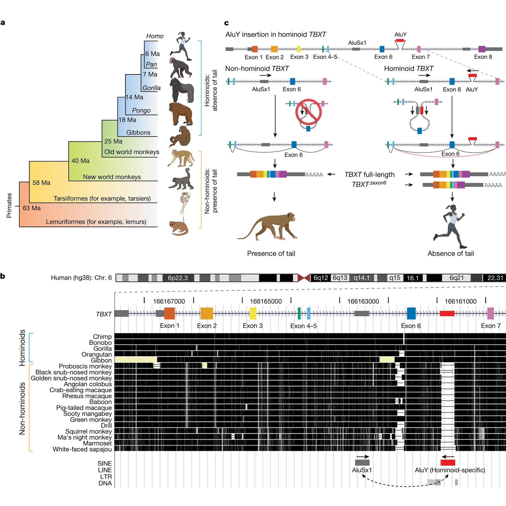
In the figure above you can see this displayed in A) which provides an overview of the presence or absence of tails in the primate family tree.
But Xia’s big discovery came when he looked at a gene, TBXT, in a genome browser (B) and he noticed that Apes have an extra sequence between exons 6 and 7 that monkeys don’t have!
This sequence was a primate specific Alu element.
Alu’s are little bits of DNA that were left behind by ancient retroviruses as they jumped in and out of our genomes.
We have about a million of these sprinkled throughout our genes and they are the most common ‘transposable element’ found in the primate genome.
They’re broadly implicated in promoting evolutionary change and the Alu element, AluY, in TBXT is no exception!
It appears that AluY collaborates with another primate Alu element, AluSx1, that’s conserved in all primates.
Panel C shows how this works:
AluY and AluSx1 bind to form a loop that excludes exon 6 during splicing and this creates a TBXT transcript that’s sometimes a bit shorter in Apes.
This exon skip liberated us from our tails!
Experiments in the paper show that removal of exon 6 in one copy of TBXT produces a range of tail lengths in mice, and with a little genetic tweaking of the other copy, the authors could produce mice that no longer had tails!
But complete removal of exon 6 in both copies of TBXT caused lethal spinal cord defects, underscoring the delicate nature of tail-loss evolution.
###
Xia B et al. 2024. On the genetic basis of tail-loss evolution in humans and apes. Nature. DOI: 10.1038/s41586-024-07095-8
Single-cell and spatial proteomics - a more refined future.
Proteomics is the study of all of the proteins produced by our cells.
This includes how they interact with one another and how all of those proteins collaborate to create the numerous tissues that make up multicellular organisms!
But, proteomics has the same exact problem that most omics approaches have as it relates to how we collect and analyze samples.
Until recently, omics studies were done on bulk material, meaning we collect a blood sample or take a tissue biopsy and then grind up all of those cells.
We then throw them on an instrument to detect everything that’s in there.
The problem with this approach is that blood (and tissues) contain many millions of cells and not all of them are the same!
What happens when you measure a sample in bulk is that all of those cells and the proteins/RNA/DNA in them get mixed with all of those things from the other cells in the sample.
This has the effect of averaging out all of the signals, meaning, you’re likely only going to be able to detect big changes within the population of cells you sampled!
Unfortunately, you might be really interested in small changes, or changes that happen gradually over time.
Because, it’s the activities of individual cells working together (but differently) that makes us who we are!
It’s also small populations of misbehaving cells in things like cancer that can cause big problems later, and it’d be super nice to detect those signals sooner rather than later!
Wouldn’t it be swell if we could do proteomics on individual cells?
Thankfully, we’re in luck!
The explosion of the field of single-cell and spatial transcriptomics (looking at RNA) has also led to methods that allow us to look at proteins at the same time.
You might be wondering why we'd care about proteins if we’re already able to look at RNA.
And that’s because RNA expression doesn’t always correlate directly with protein abundance!
So, you can have lots of an mRNA in a cell, and a little of its translated protein, or vice versa depending on what a cell is doing at any given time!
This means that the two techniques are very complementary, and if you’re already doing transcriptomics, most methods allow you to throw in a bunch (50-100) of antibodies to also detect proteins you might be interested in.
But, what if you want to GET ALL OF THE PROTEINS?!?!?!
If you’re a proteomics Cookie Monster, you’re also in luck!
We also have LCMS based methods that take an unbiased approach to protein detection.
And when paired with fancy new separation and capture techniques, we can use LCMS to detect and quantify all of the proteins in single cells or within a tissue section.
While these techniques are still in the earliest stages of development, they offer the promise of a more precise future for increasing our understanding of the biology behind health and disease!
The field of molecular biology was born in 1941 through the marriage of genetics and biochemistry.
This, to this day, is not a very happy marriage.
Both sides tolerate one another, but the biochemists lean on function and the geneticists lean on math and statistics.
The progeny, or molecular biologists, fall in the middle, trying to muffle the yelling and screaming of the other two, but this diversity of ideas is actually what makes science great - even if mom and dad fight sometimes!
But, before we dig into the birth of this dysfunctional family, it is important to highlight that in the 1900's, the idea of a 'gene' was an abstract one.
We all know Mendel and his peapods, that traits are inherited and it was thought that this was all controlled by genes, but 'how' any of that worked biologically was essentially a mystery.
George Beadle was fascinated with the 'how' and spent many years in a Drosophila (fruit fly) lab trying to connect pigments to whatever a gene was.
And he rightly hypothesized it involved biochemical pathways.
He realized that approaching the problem from the perspective of the end product, the pigment, was wrong.
And this meant he had to figure out how to break the 'gene' and link it directly to biochemistry.
But doing that in a complex multicellular organism like a fruit fly was going to be impossible so he switched to a much simpler one: Neurospora!
Now, Neurospora, being a fungus, has certain features that made it ideal for this project.
Fungi are haploid (1 copy of the genome per cell, not 2) for a good portion of their life and heritable genetic changes are easy to track in their offspring because you don’t have to worry about any compensatory interference from an alternate working copy!
Beadle realized he could create mutations in fungi and then link those to biochemical processes.
But how do you make mutations in genes in 1941?
With X-rays!
So, he irradiated a bunch of haploid Neurospora and then grew them on different types of food:
One that had everything they needed to live (complete), and one that did not (minimal).
Once he found mutants that could grow on complete but not minimal, he added back individual components to the minimal food to figure out what the fungi couldn't make anymore.
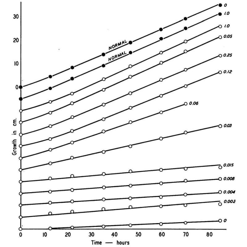
What he found is shown in the figure above, which displays the growth rate of normal Neurospora (black dots) and a mutant (open dots) that couldn’t make vitamin B6 anymore.
This mutant could be saved though, and its growth rate controlled based on how much B6 (numbers) was added back to the food.
Given enough B6, the mutant could grow just as well as the normal one!
This might seem super basic, but it was the first clear evidence that linked a biochemical process directly to a heritable gene - the rest is molecular biology!
###
Beadle GW and Tatum EL. 1941. Genetic control of biochemical reactions in Neurospora. PNAS. DOI: 10.1073/pnas.27.11.499
Were you forwarded this newsletter?
LOVE IT.
If you liked what you read, consider signing up for your own subscription here: